[Deep Learning] 1. Introduction
Introduction
AI is good at solving tasks that are intellectually difficult for humans, but conversely, it is not good at solving tasks that are easy for humans but difficult to describe formally. (e.g., recognizing spoken words or faces in images.)
The solution to these intuitive problems is to have computers learn from experience and understanding of the world. (in terms of a hierarchy of concepts, with each concept defined through its relation to simpler concepts.) If you draw a graph of how the hierarchy of concepts is done, it will be very deep, so this approach is called AI deep learning.
Hard-code knowledge
The key is to get informal knowledge about the world into a computer. One approach, called knowledge base, have sought to hard-code knowledge about the world in formal languages… but none has led to a major success. (e.g., Cyc(Lenat and Guha, 1989) do not capture the person Fred while shaving.)
Machine learning
Thus, the capability to acquire their own knowledge, by extracting patterns from raw data, is needed. a.k.a machine learning.
Simple machine learning algorithms
The famous & simple ML algorithms are logistic regression, which can determine whether to recommend cesarean delivery, and naive Bayes, which can separate legitimate e-mail from spam. However, these simple ML algorithms depend heavily on the representation(or feature in it) of the data, so they cannot influence how features are defined in any way.
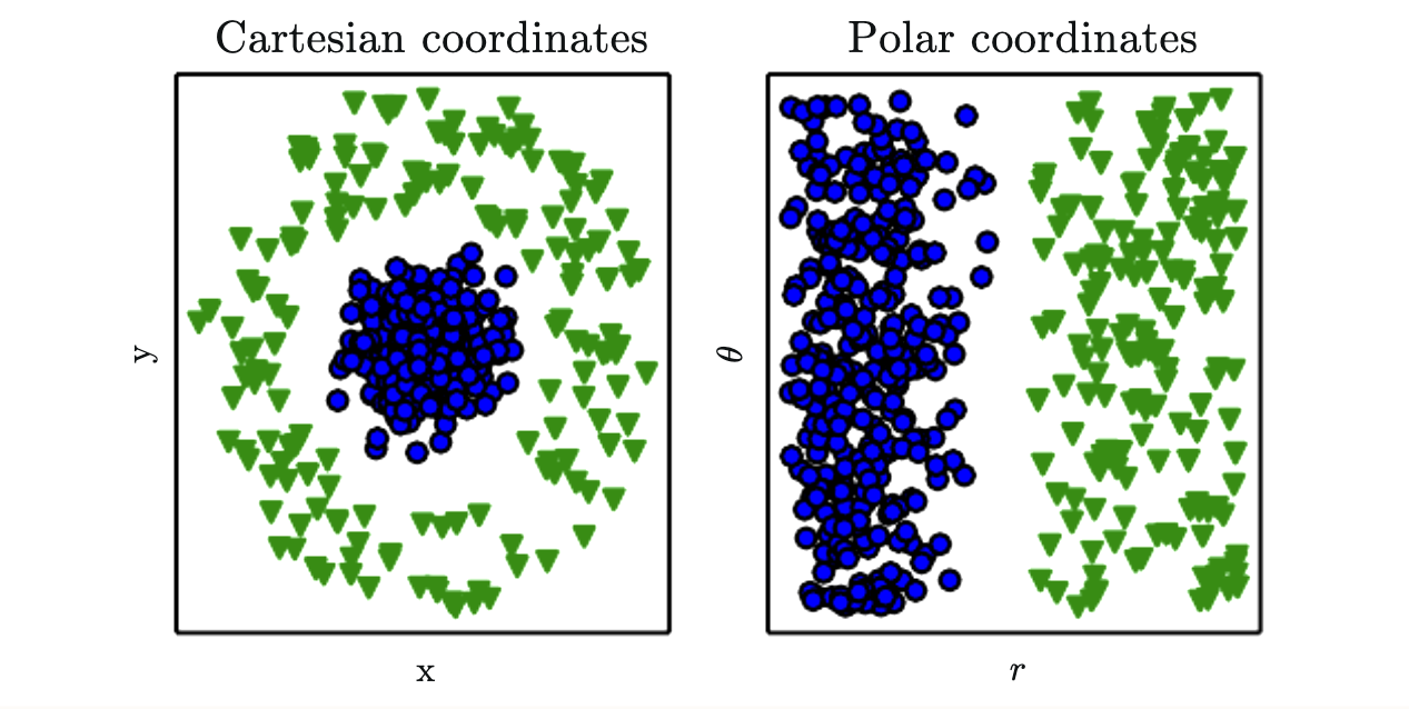 Figure 1.1: Example of different representations
In other words, many AI tasks can be solved by designing the right set of features, like figure 1.1. (e.g., a useful feature for speaker identification is the size of the vocal tract1) However, of course, it is difficult to know what features should be extracted.
Representation learning
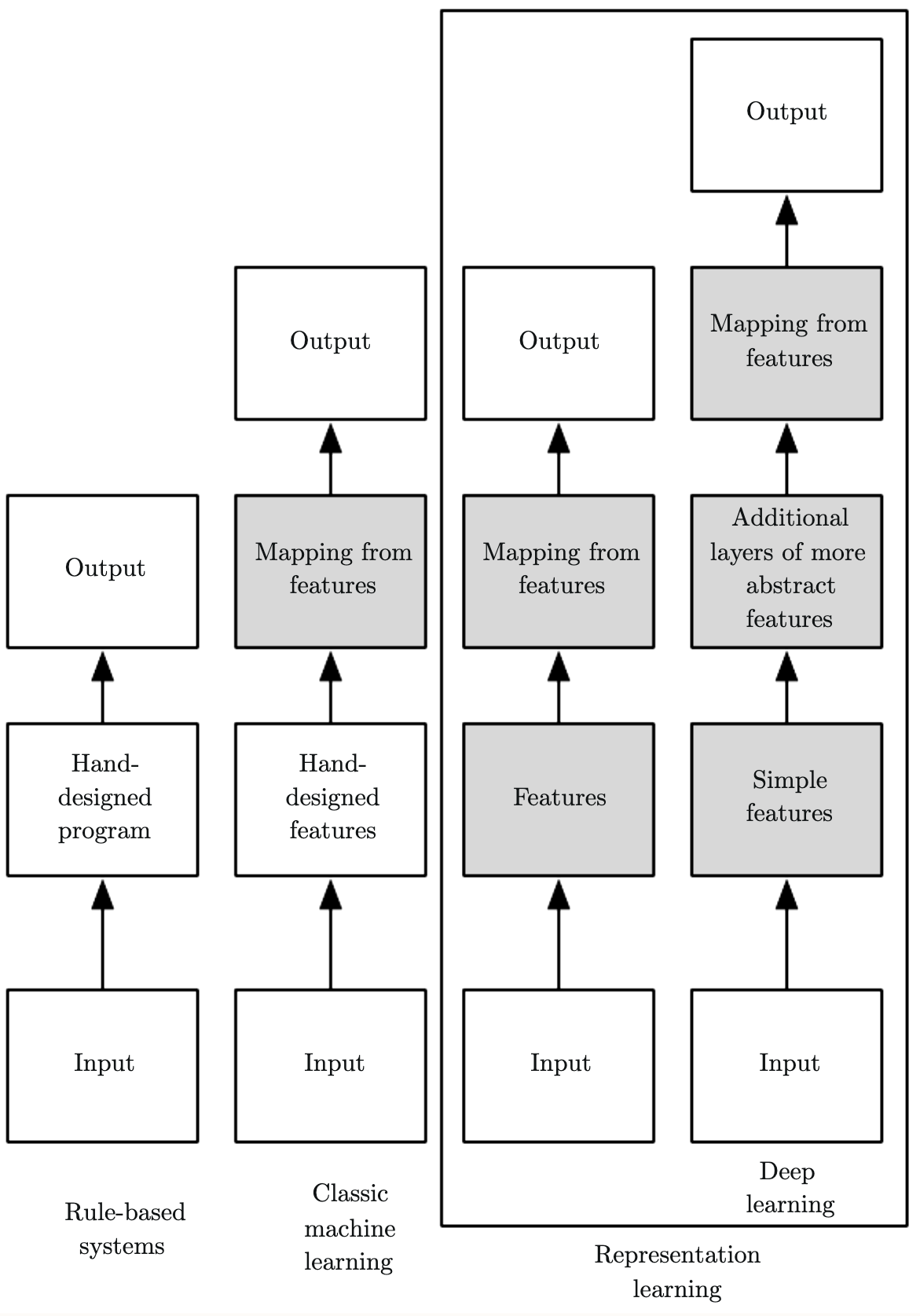
One solution to this problem is representation learning. This discovers not only the mapping but also the representation itself. It allows AI systems to rapidly adapt to new tasks, with minimal human intervention. The quintessential2 example of a representation learning algorithm is the autoencoder3.
When designing features or algorithms for learning features, our goal is usually to separate the factors4 of variation, which include the speaker’s age, their sex, their accent and the words they are speaking. The major source of difficulty in many real-world AI applications comes from these factors of variation.
Deep learning
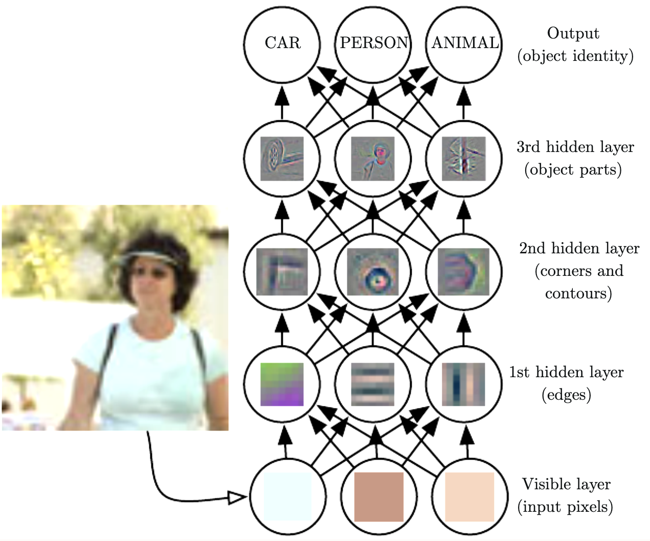 Figure 1.2: Illustration of a deep learning model. There is a series of hidden layers that extracts increasingly abstract features from the image.
Of course, it is difficult to extract such high-level & abstract features, such as a speaker’s accent, from raw data. Deep learning solves this central problem in representation learning by introducing representations that are expressed in terms of other, simpler representations. (figure 1.2) A deep learning system can represent the concept of an image of a person by combining simpler concepts, such as corners and contours, which are in turn defined in terms of edges.
The quintessential example of a deep learning model is the feedforward deep network, called multilayer perceptron (MLP)5.
Then, how “deep” can be measured? There are two main ways of measuring the depth of a model.
- based on the number of sequential instructions that must be executed.
- Used by deep probabilistic models, regards as the depth of the graph describing how concepts are related to each other.
It is not always clear which of these two is most relevant, nor there is a consensus about how much depth a model requires to qualify as “deep”. However, it can be safely regarded as the study of the models that involve a greater amount of composition of either learned functions or learned concepts (than traditional ML).
Deep learning is a particular kind of ML that achieves great performance by representing the world, with relations to simpler concepts. The figure below would help understand what deep learning is.
1.1 Who Should Read This Book?
Students and beginners.
- Part I introduces basic mathematical tools and ML concepts.
- Part II describes the most established deep learning algorithms.
- Part III describes more speculative ideas that are believed to be important.
1.2 Historical Trends in Deep Learning
The below is a few key trends of deep learning:
- Deep learning has had a long and rich history, but has gone by many names, reflecting different philosophical viewpoints, and has waxed and waned in popularity.
- Deep learning has become more useful as the amount of available training data has increased.
- Deep learning models have grown in size over time as computer infrastructure (both hardware and software) for deep learning has improved.
- Deep learning has solved increasingly complicated applications with increasing accuracy over time.
1.2.1 The Many Names and Changing Fortunes of Neural Networks
Many of readers may heard of deep learning as an new technology but the history starts from the 1940s. Cybernetics in the 1940s-1960s, connectionism in the 1980s-1990s and deep learning beginning in 2006.
Some earliest learning algorithms were intended for biological learning, how learning happens or could happen in the brain. So, Artificial neural networks (ANNs) was one of the names that deep learning has gone by.
First wave
However, the modern term deep learning goes beyond the neuroscientific perspective. It appeals to a more general principle of learning multiple levels of composition. The first wave of NN research was cybernetics, learn a set of weights $w_1, \dots, w_n$ and compute the output $f(\mathbf{x, w}) = x_1w_1+\cdots+x_nw_n$ .
- 1940s:
- McCulloch-Pitts neuron, which could recognize two different categories.
- 1950s:
- Perceptron, which could learn the weights that defined the categories given examples of inputs from each category.
- Adaptive linear element (ADALINE), which simply returned the value of $f(\mathbf{x})$ itself to predict a real number.
ADALINE was a special case of SGD, variants of which remain the dominant today. Perceptron and ADALINE are called linear models which cannot learn the XOR function. (e.g., $f([0,1], \mathbf{w})=1$ and $f([1,0], \mathbf{w})=1$ but $f([1,1], \mathbf{w})=0$ and $f([0,0], \mathbf{w})=0$.)
Today, neuroscience is an important source of inspiration but no longer predominant guide because we do not have enough information about the brain.
However, we can draw some guidelines from neuroscience:
- The neocognitron(Fukushima, 1980) later became the basis for the modern convolutional network(LeCun et al., 1998).
- Most Neural networks today are based on the rectified linear unit.
- and so on.
It remains as a separate field.
Second wave
In the 1980s, the second wave of NN research emerged via a movement called connectionism, or parallel distributed processing (Rumelhart et al., 1986c; McClelland et al., 1995). The central idea in connectionism is that a large number of simple computational units can achieve intelligent behavior when networked together.
Another concept is that of distributed representation, which says that each input should be represented by many features. (e.g., red truck, red car, … rather than just car, red, blue, …). This distributed representation will be dealt in detain in chapter 15.
Another major accomplishment was the successful use of back-propagation, which is famous to people I think.
In 1990s, Hochreiter and Schmidhubler (1997) introduced the long short-term memory (LSTM) for dealing with long sequences, described in section 10.7. LSTM is still widely used today, also at Google.
However, the second wave ended in mid-1990s because AI research did not satisfy the expectations and Other fields, Kernel machines and graphical models, achieved good results. So, the popularity of NN declined until 2007. During this time, CIFAR keep NN research alive via its Neural computation and Adaptive Perception (NCAP).
Third wave
The third wave began in 2006. At this time, deep neural networks outperformed competing AI systems based on other machine learning technologies as well as hand-designed functionality.
The third wave began with a focus on new unsupervised learning techniques and the ability of deep models to generalize well from small datasets, but today there is more interest in much older supervised learning algorithms and the ability of deep models to leverage large labeled datasets.
1.2.2 Increasing Dataset Sizes
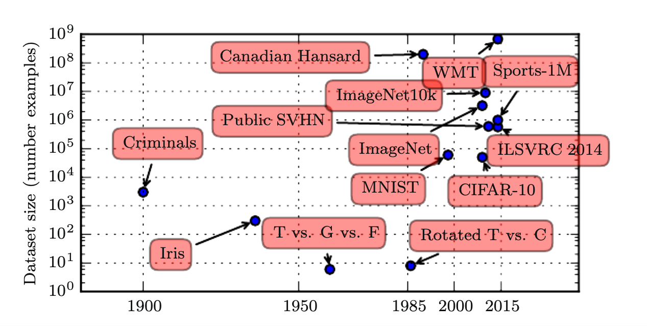 FIgure 1.8: Increasing dataset size over time.
The size of benchmark datasets has expanded remarkably over time. This increasing dataset size has made ML much easier because the key burden of statistical estimation has been considerably lightened.
Unsupervised or semi-supervised learning are important research area to achieve successful performance with datasets smaller than 10 million labeled examples.
1.2.3 Increasing Model Sizes
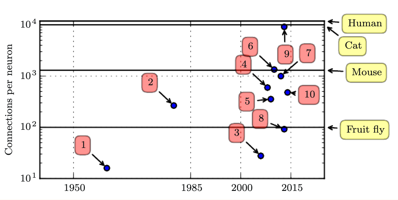 Figure 1.10: Number of connections per neuron over time.
As we can see here model size increases over time, due to the availability of faster CPUs & GPUs.
Each of them is:
- Adaptive linear element (Widrow and Hoff, 1960)
- Neocognitron (Fukushima, 1980)
- GPU-accelerated convolutional network (Chellapilla et al., 2006)
- Deep Boltzmann machine (Salakhutdinov and Hinton, 2009a)
- Unsupervised convolutional network (Jarrett et al., 2009)
- GPU-accelerated multilayer perceptron (Ciresan et al., 2010)
- Distributed autoencoder (Le et al., 2012)
- Multi-GPU convolutional network (Krizhevsky et al., 2012)
- COTS HPC unsupervised convolutional network (Coates et al., 2013)
- GoogLeNet (Szegedy et al., 2014a)
1.2.4 Increasing Accuracy, Complexity and Real-World Impact
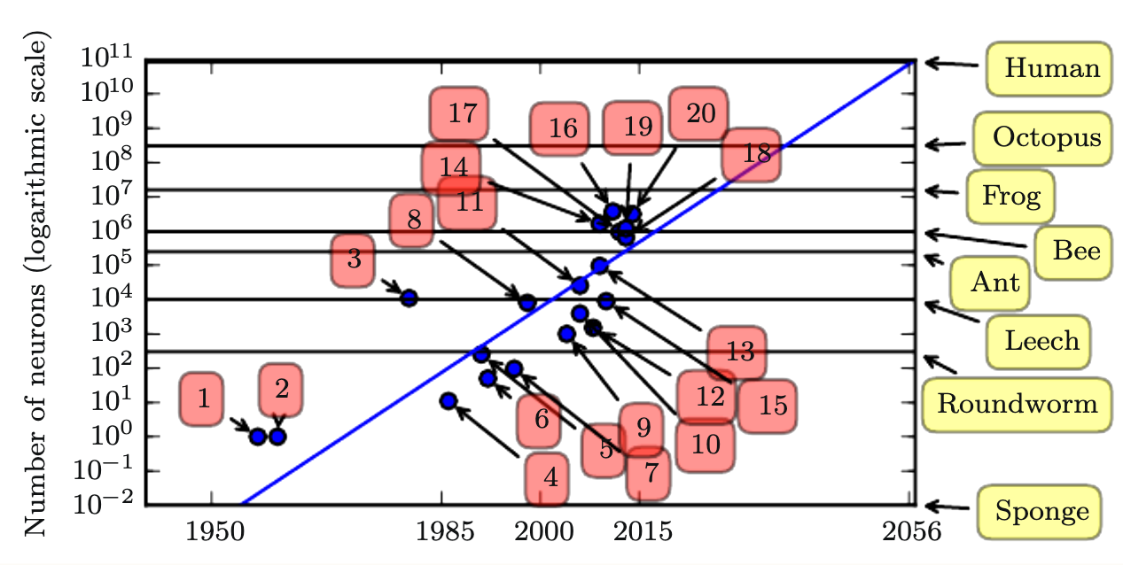 Figure 1.11: Increasing neural network size over time.
The earliest deep models were used to recognize individual objects in tightly cropped, extremely small images. However, modern object recognition networks process rich high-resolution photographs and do not have a requirement that the photo be cropped near the object to be recognized (Krizhevsky et al., 2012).
As figure 1.11 shows, NN size has increased exponentially. (Caution: figure 1.10 shows the number of connections and figure 1.11 shows the number of neurons.)
As the model size goes on, accuracy of deep networks have also increased.
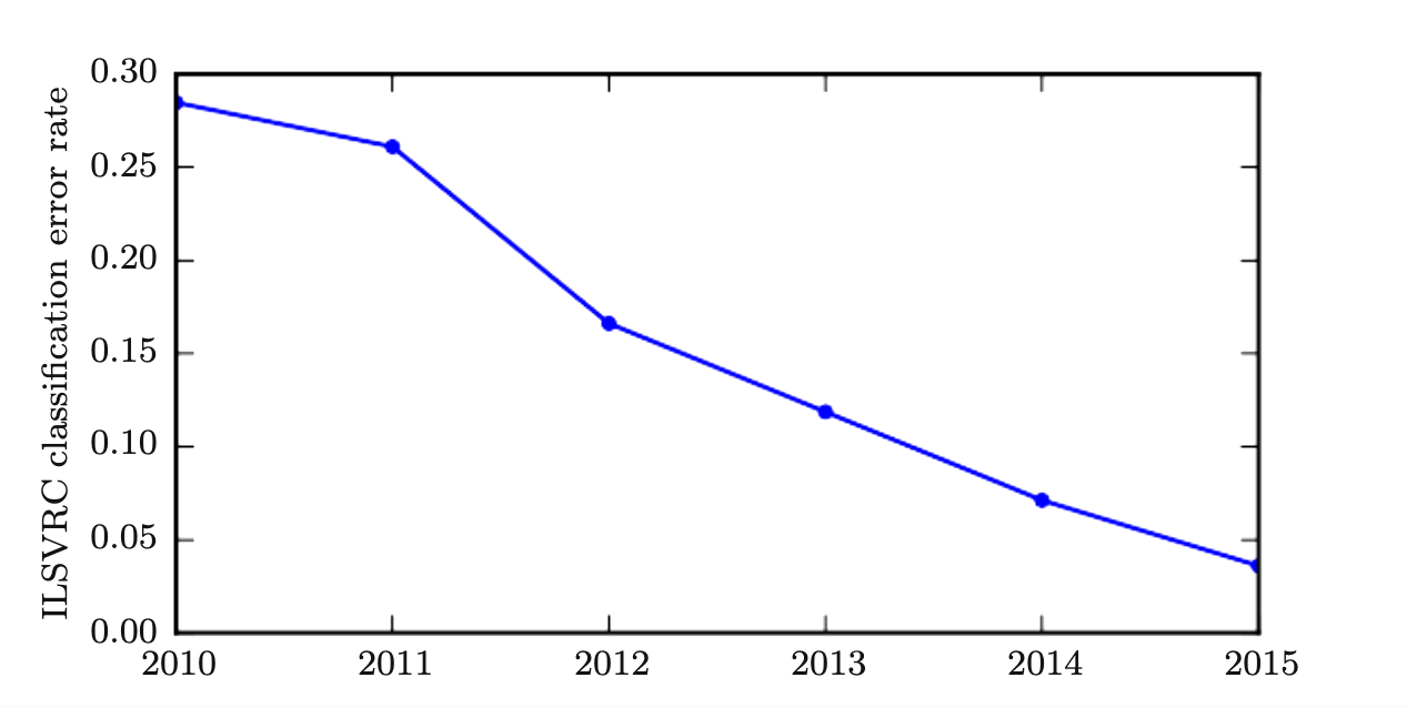 Figure 1.12: Decreasing error rate over time.
성대 ↩︎
본질적인 ↩︎
An encoder encodes the input data into a different representation, and a decoder converts it back into the original format. ↩︎
Can be thought of as concepts or abstractions that help us make sense of the rich variability in the data. ↩︎
Which is just a mapping some set of input values to output values, which is formed by many simpler functions. ↩︎
